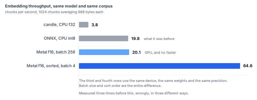
The first time I benchmarked GPU embedding against the CPU path, the GPU lost by a factor of 1.7. The second time it tied. The third time it lost again, differently.
The fourth time it was 3.3× faster than the CPU and 3.2× faster than the ONNX runtime we were actually using. Nothing about the hardware changed between the third and fourth runs.
Here is what I had wrong each time, because the mistakes are more transferable than the result.
What I was trying to do
Indexing a code corpus means embedding a few hundred thousand chunks, and on this machine it was taking most of an hour per large repository while pinning every core. The embedding library uses ONNX Runtime on CPU. There's an Apple GPU sitting right there doing nothing.
So: same model, same weights, run the forward pass through Metal instead. Two hundred lines. The kind of change that should take an afternoon.
It took considerably longer than an afternoon, and all of the extra time went into finding out that my measurements were lying to me.
Wrong the first time: I used chunks that were too big
My first benchmark fed 1200-byte chunks, because that was near the model's 512-token limit and it felt like the honest stress test. The GPU came out 1.7× slower than the CPU and I nearly stopped there.
The problem is that attention memory grows with the square of sequence length. At batch 256 and 512 tokens, the intermediate tensors work out to roughly 3.2 GB, which on unified memory means you spend the run moving data rather than computing on it. The GPU wasn't slow. It was thrashing.
Then I went and looked at what the indexer actually produces. Mean chunk size across the corpus was 688 bytes, about 250 tokens. Half of what I'd been testing with.
That's the mistake in one line: I benchmarked the worst case and concluded something about the average case. Once I re-ran at 688 bytes the GPU stopped losing.
If you take one thing from this post, take that one. Measure the distribution your system actually produces before you pick a benchmark input.
Wrong the second time: I never tested f16
The second round I ran everything in f32 because it was what worked, and reported that Metal was about even with ONNX. Even is not a reason to add two hundred lines of code, so I nearly shelved it again.
I hadn't tested half precision. Not because I'd ruled it out. I tried once, it crashed, and I moved on.
The crash was mine. My mean-pooling step built the attention mask as f32 and multiplied it against the hidden states:
One line. It had cost me an entire configuration.
And the honest footnote: f16 turned out to buy only about 3% at the batch size I ended up shipping. It's 19% at batch 256. That distinction matters, and I'll come back to it. The point here is that "I tried it and it crashed" is not the same as "I tested it," and I had been treating them as the same.
Wrong the third time: I sorted by the wrong length
Batches pad to the longest sequence in them, so grouping similar-length inputs together cuts wasted computation. Standard trick. I sorted chunks by byte length and re-ran.
Padding went up.
The corpus is Korean-commented code, and in it byte length barely predicts token length. Hangul costs three bytes a syllable and about half a token; a long identifier costs the reverse. Sorting by bytes had been grouping the wrong things together, so the batches it produced were no tighter than random ones. Sorting by token count instead:
| batch | order | wall clock | chunks/s | padded tokens |
|---|---|---|---|---|
| 4 | unsorted | 18.9s | 54.1 | 220,396 |
| 4 | token-sorted | 15.9s | 64.6 | 196,688 |
| 64 | unsorted | 32.3s | 31.7 | 266,112 |
| 64 | token-sorted | 21.0s | 48.8 | 204,736 |
| 256 | unsorted | 44.5s | 23.0 | 290,560 |
| 256 | token-sorted | 29.9s | 34.2 | 230,656 |
Two things fall out of that table, and I only expected one of them.
The thing I didn't expect: small batches win
Every instinct says larger batches are better on a GPU. More parallelism, fewer kernel launches, better occupancy.
Batch 4 beat batch 256 by 1.9× after sorting, and by 2.4× before it. The padded-token column explains most of it: a batch of 256 has to pad everything up to the longest member, and with 256 members you're almost guaranteed a long one. Batch 4 pads to the longest of four. That's 290k tokens of work versus 196k for the identical corpus, and about a third of the larger batch's compute is spent on padding that gets multiplied by zero and thrown away.
The rest is bandwidth. At these sizes the model is small enough that we're not compute-bound at all; we're moving weights and activations. Bigger batches move more.
This is also why f16 gave 19% at batch 256 and only 3% at batch 4. Halving the precision helps when you're bandwidth-bound in the way large batches are. At batch 4 there's less to move and the win mostly evaporates. The optimisations interact, and testing them one at a time on the wrong batch size tells you nothing about the combination you'll ship.
What it looks like in production
Wired into the actual indexer, on one repository of 406 files:
| ONNX int8 | Metal f32 | |
|---|---|---|
| cold index | 294s | 152s |
| CPU time consumed | 1,736s | 7.2s |
| Pass@1 / Pass@5 / Pass@10 | 26.8 / 42.9 / 42.9 | identical |
| MRR | 0.332 | identical |
The CPU-time row is the one that changed how the machine feels. The ONNX path saturated every core for the duration, and you could not comfortably use the laptop while an index was building. The Metal path uses about seven seconds of CPU across the whole run.
Quality is identical to three decimal places, which is what you'd expect from the same weights at higher precision, but I checked rather than assumed. Retrieval quality is exactly the sort of thing that degrades quietly.